A data set contains longitudinal data of mean hourly wages along with several demographic variables of Americans from the National Longitudinal Survey of Youth (NLSY79) held by the U.S. Bureau of Labor Statistics from Round 1 (1979 survey year) to Round 28 (2018 survey year). The cohort provided in this data set is the highest grade completed, up to 12th grade, and participated in at least five rounds of surveys.
Format
A tsibble with 103,994 rows and 15 variables:
- id
A unique individual's ID number. This is the
keyof the data.- year
The year the observation was taken. This could be the
indexof the data.- wage
The mean of the hourly wages the individual gets at each of their different jobs. The value could be a weighted or an arithmetic mean. The weighted mean is used when the information of hours of work as the weight is available. The mean hourly wage could also be a predicted value if the original value is considered influential by the robust linear regression as part of data cleaning.
- age_1979
The age of the subject in 1979.
- gender
Gender of the subject, FEMALE and MALE.
- race
Race of the subject, NON-BLACK,NON-HISPANIC; HISPANIC; BLACK.
- hgc
Highest grade completed.
- hgc_i
Integer of highest grade completed.
- yr_hgc
The year when the highest grade completed.
- njobs
Number of jobs that an individual has.
- hours
The total number of hours the individual usually works per week.
- is_wm
Whether the mean hourly wage is weighted mean, using the hour work as the weight, or regular/arithmetic mean. TRUE = is weighted mean. FALSE = is regular mean.
- is_pred
Whether the mean hourly wage is a predicted value or not.
Source
The U.S. Bureau of Labor Statistics. (2021, January 6). National Longitudinal Survey of Youth 1979. https://www.nlsinfo.org/content/cohorts/nlsy79/get-data
Examples
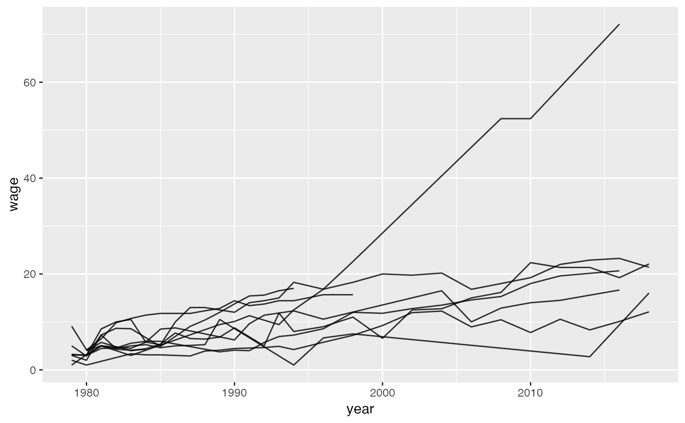
# data summary wages#> # A tsibble: 103,994 x 13 [!] #> # Key: id [5,931] #> id year wage age_1979 gender race hgc hgc_i yr_hgc njobs hours is_wm #> <fct> <int> <dbl> <int> <fct> <fct> <fct> <int> <int> <int> <int> <lgl> #> 1 2 1979 3.85 20 FEMALE NON-B… 12TH… 12 1985 1 35 FALSE #> 2 2 1980 4.57 20 FEMALE NON-B… 12TH… 12 1985 1 NA FALSE #> 3 2 1981 5.14 20 FEMALE NON-B… 12TH… 12 1985 1 NA FALSE #> 4 2 1982 5.71 20 FEMALE NON-B… 12TH… 12 1985 1 35 FALSE #> 5 2 1983 5.71 20 FEMALE NON-B… 12TH… 12 1985 1 NA FALSE #> 6 2 1984 5.14 20 FEMALE NON-B… 12TH… 12 1985 1 NA FALSE #> 7 2 1985 7.71 20 FEMALE NON-B… 12TH… 12 1985 1 NA FALSE #> 8 2 1986 7.69 20 FEMALE NON-B… 12TH… 12 1985 1 NA FALSE #> 9 2 1987 8.79 20 FEMALE NON-B… 12TH… 12 1985 1 NA FALSE #> 10 2 1988 6.67 20 FEMALE NON-B… 12TH… 12 1985 2 NA FALSE #> # … with 103,984 more rows, and 1 more variable: is_pred <lgl>#> Warning: package ‘dplyr’ was built under R version 4.0.2#> #>#> #> #>#> #> #>library(tsibble) wages_ids <- key_data(wages) %>% select(id) wages %>% dplyr::filter(id %in% sample_n(wages_ids, 10)$id) %>% ggplot() + geom_line(aes(x = year, y = wage, group = id), alpha = 0.8)