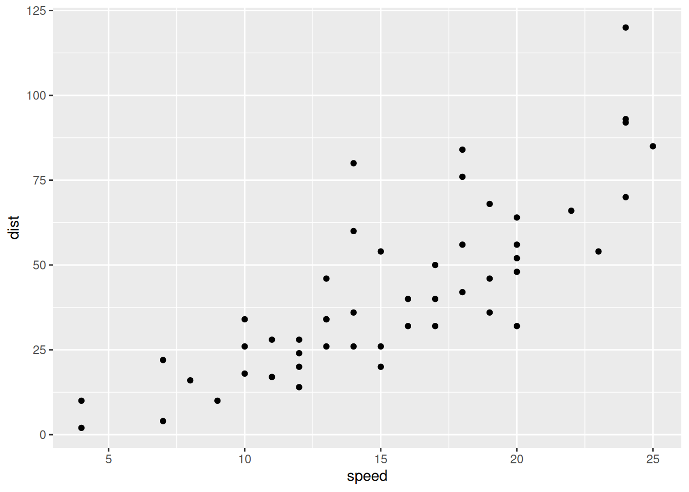
library(ggplot2)
ggplot(cars, aes(speed, dist)) +
  geom_point()
Welcome to the LearR Academy module on Linear Regression! This module is designed to introduce you to the concepts and techniques of linear regression, an widely used tool in the field of statistics, data science, and machine learning. Through this module, you will explore the mathematical principles underlying linear regression, learn how to build and evaluate models using R, and understand the practical applications of these models in real-world scenarios. Whether you are predicting housing prices or forecasting sales, this module will equip you with the skills and knowledge to leverage the power of linear regression for insightful data analysis and informed decision-making.
13 December 2024
Linear regression is a statistical method used to model the relationship between a dependent variable and one or more independent variables. It aims to find the best-fitting linear relationship that describes how the dependent variable changes in response to the independent variable(s). This technique is of key importance in statistics and data science and is used extensively for predictive analysis.
Simple linear regression refers to fitting a straight line to a set of data points to model the relationship between a single independent variable and a dependent variable. The equation of a simple linear regression model is given by: \(y = \beta_0 + \beta_1x + \epsilon\), where \(y\) is the dependent variable, \(x\) is the independent variable, \(\beta_0\) is the intercept, \(\beta_1\) is the slope, and \(\epsilon\) is the error term that follows a normal distribution with zero mean and constant variance \(\sigma^2\).
The Pearson correlation coefficient (\(r\)) is a measure of the strength and direction of association between two continuous variables. It ranges from -1 to 1, where:
The Pearson correlation coefficient is calculated using the following formula:
\[ r_{x,y} = \frac{\sum_{i_1}^{n}{(x_i-\bar{x})(y_i-\bar{y})}} {\sqrt{\sum_{i=1}^{n}{(x_i-\bar{x})^2}}\sqrt{\sum_{i=1}^{n}{(y_i-\bar{y})^2}}} \]
where:
Consider the mtcars dataset. Compute the the Pearson correlation coefficient between mpg (miles per gallon) and hp (horsepower).
Consider the mtcars dataset. Create a scatter plot with a regression line considering the variables mpg (miles per gallon) and hp (horsepower).
# Load the dataset
data(mtcars)

# Perform linear regression
model <- lm(mpg ~ hp, data = mtcars)

# Summary of the model
summary(model)
Call:
lm(formula = mpg ~ hp, data = mtcars)

Residuals:
    Min      1Q  Median      3Q     Max
-5.7121 -2.1122 -0.8854  1.5819  8.2360

Coefficients:
            Estimate Std. Error t value Pr(>|t|)
(Intercept) 30.09886    1.63392  18.421  < 2e-16 ***
hp          -0.06823    0.01012  -6.742 1.79e-07 ***
---
Signif. codes:  0 '***' 0.001 '**' 0.01 '*' 0.05 '.' 0.1 ' ' 1

Residual standard error: 3.863 on 30 degrees of freedom
Multiple R-squared:  0.6024,    Adjusted R-squared:  0.5892
F-statistic: 45.46 on 1 and 30 DF,  p-value: 1.788e-07
Congratulations! This is the end of the Linear Regression with R module!